Particle Detectors

Chapter 1 — Gaseous-filled detectors working principle

Summary

1. Introduction
2. Operating regions
3. Operating modes

1. Introduction

There are three main kinds of radiation detectors:

• Scintillation detectors
• Semiconductor detectors
• Gas-filled detectors

Here we focus on gas-filled detectors.

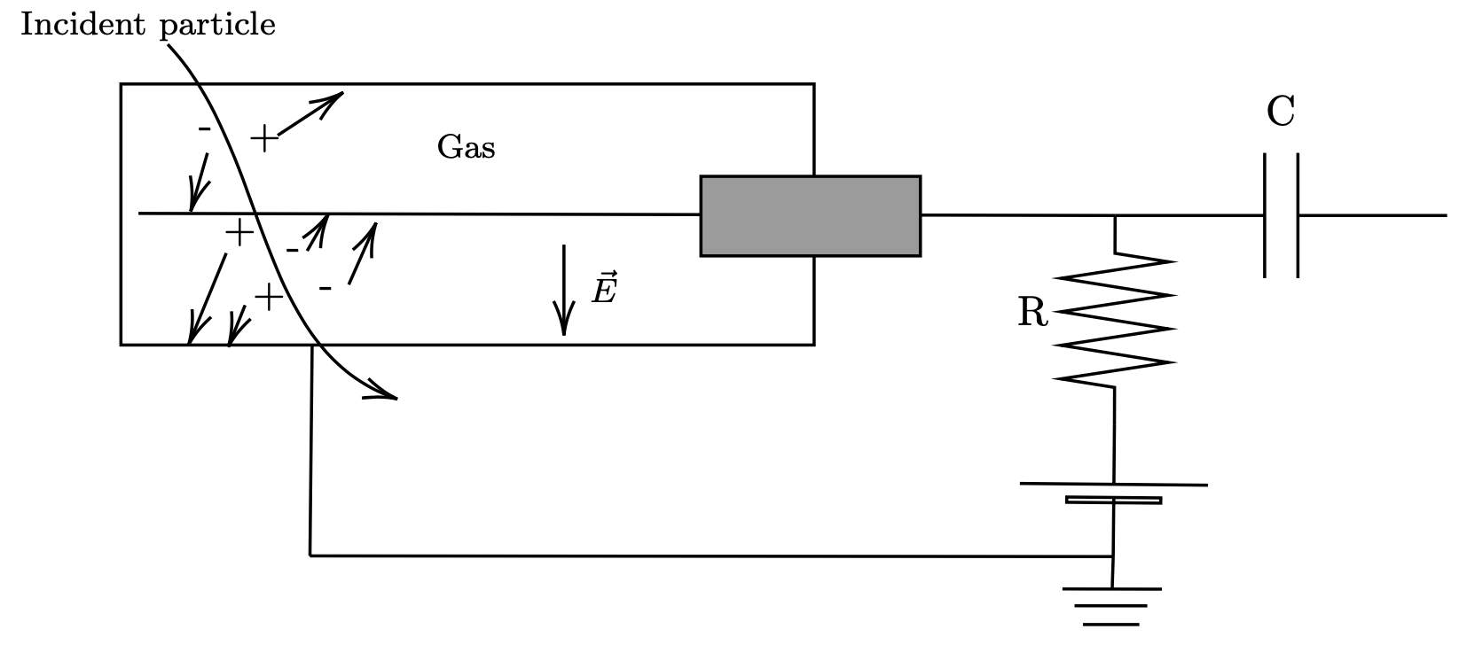
Detecting radiation consists of converting the energy deposited by the radiation into an electrical signal. In a gas-filled detector, the incident radiation ionizes the gas, directly or indirectly. The resulting charges drift under the electric field and induce a measurable electrical signal.

Neutrons are not directly ionizing particles. They can therefore be detected by first converting them into charged, ionizing particles through suitable nuclear reactions.

The operating voltage of a gas-filled detector determines its operating regime and therefore the type of detector that can be built.

2. Operating regions

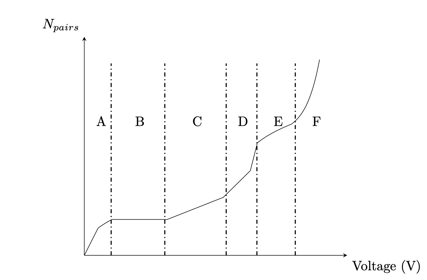
The pulse amplitude of a gas-filled detector depends on the applied high voltage. Several operating regions can be identified.

Region A — Recombination region

At low voltage, the electric field is too weak to efficiently collect the charges. Recombination dominates over charge collection.

As the voltage increases, recombination decreases and the pulse amplitude increases.

This region is not suitable for detector operation.

Region B — Ionization region

The voltage is high enough for recombination to become negligible, but too low for avalanche multiplication to occur.

The number of collected charges is therefore equal to the number of charges initially generated:

$$N_{\text{induced}} = N_{\text{generated}}$$

The pulse amplitude is proportional to the energy deposited by the radiation.

The current is very low, of the order of

$$10^{-13}\,\text{A}$$

This region is used for ionization fission chambers, which can operate at high neutron fluxes without requiring charge multiplication.

Region C — Proportional region

At higher voltage, the electric field becomes strong enough to produce secondary ionization and an avalanche effect.

The number of induced charges becomes

$$N_{\text{induced}} = kN_{\text{generated}}, \qquad k>1$$

The pulse amplitude remains proportional to the energy deposited by the particle.

The current is significantly higher, approximately

$$10^{-6} - 10^{-3}\,\text{A}$$

This region is used by proportional counters, particularly at lower fluxes where charge multiplication is useful.

Region D

Charge collection becomes disturbed and proportionality is lost.

Region E — Geiger plateau

The detector operates in the Geiger region. The collected charge is limited by the characteristics of the detector rather than by the initial ionization.

Region F

The discharge becomes unstable.

3. Operating modes

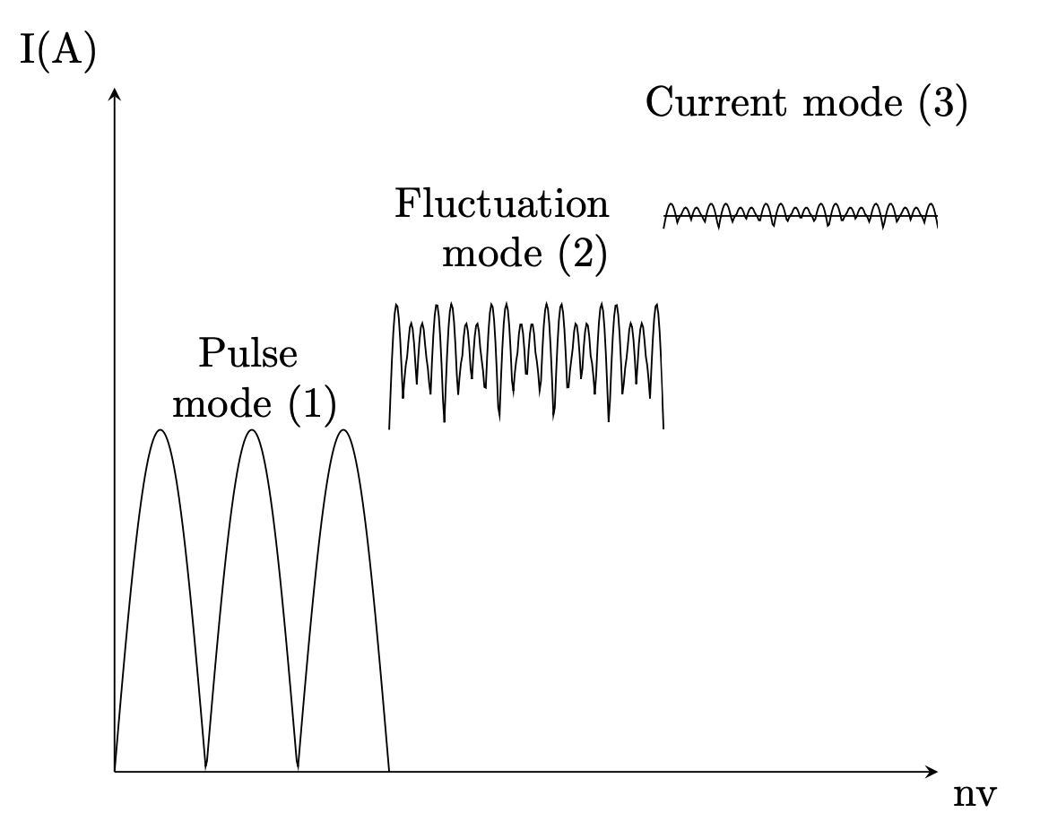
The appropriate measurement mode depends on the incident neutron flux.

Three main modes can be distinguished:

Flux region	Measurement mode	Principle
Low flux	Pulse mode	Individual pulses are measured
Intermediate flux	Fluctuation / Campbell mode	Statistical fluctuations are measured
Very high flux	Current mode	Continuous detector current is measured

At low counting rates, individual pulses can be discriminated and processed.

As the counting rate increases, pulses begin to overlap and form a fluctuating signal. At very high rates, the signal becomes essentially continuous.

3a. Pulse mode

Pulse mode is associated with low neutron flux.

Individual pulses are measured by observing the voltage across a resistor-capacitor circuit. Each pulse corresponds to a collected charge $Q$ over a characteristic duration $T$.

CPNB detectors operate solely in this mode.

Two cases are particularly important.

Fast circuit: $RC \ll T$

The measurement circuit is very fast and reproduces the initial pulse accurately.

However, measuring the maximum voltage becomes difficult because the capacitor does not have enough time to reach its maximum value. The sensitivity to pulse fluctuations is also relatively limited.

Slow circuit: $RC \gg T$

The charge $Q$ passes progressively through the resistor and reaches a maximum voltage

$$V_{\max} = \frac{Q}{C}$$

at approximately

$$t=T$$

The voltage then decreases exponentially:

$$V(t) \propto e^{-t/RC}$$

Measuring the maximum voltage is easier because it is proportional to $Q$, which itself is proportional to the energy deposited by the incoming particle.

The disadvantage is pulse pile-up: at high particle rates, the long exponential decay can cause successive pulses to overlap.

3b. Campbell mode

For counting rates above approximately

$$10^5\ \text{cps}$$

individual pulses become increasingly difficult to distinguish.

Campbell’s sampling theorem can then be used to describe the detector signal statistically.

Two modes are particularly useful:

• Current mode
• Fluctuation mode

Current mode

Only the continuous component of the signal is considered.

Using Campbell’s theorem of order 1, the average current can be related to the incident neutron flux:

$$\langle I\rangle = K_I \Phi$$

where:

• $\langle I\rangle$ is the average continuous current, in A.
• $K_I$ is the detector sensitivity in A per unit thermal neutron flux.
• $\Phi$ is the thermal neutron flux, in $\text{n}\cdot\text{cm}^{-2}\cdot\text{s}^{-1}$.

Fluctuation mode

Instead of the average current, we consider its fluctuations.

Using Campbell’s theorem of order 2:

$$\operatorname{Var}(I) = K_F \Phi \times C$$

where:

• $\operatorname{Var}(I)$ is the variance of the current, in $\text{A}^2$.
• $K_F$ is the detector sensitivity in fluctuation mode, in $\text{A}^2\cdot\text{s}$ per unit thermal neutron flux.
• $C$ is a constant related to the detector pulse response, in $\text{s}^{-1}$.
• $\Phi$ is the thermal neutron flux, in $\text{n}\cdot\text{cm}^{-2}\cdot\text{s}^{-1}$.

---

Chapter 2 — Charged particle detector

Let’s consider the example of a Geiger-Müller detector.

2.1 — Theory of the Geiger-Müller detector

Coming soon.

2.2 — Electronic part

2.2.1 — General structure

The detector electronics can be represented as a chain:

$$\text{Boost Converter} \rightarrow \text{GM Tube} \rightarrow \text{Inverter} \rightarrow \text{Pulse Stretcher} \rightarrow \text{Piezo Speaker}$$

with a parallel path:

$$\text{Pulse Stretcher} \rightarrow \text{Filter} \rightarrow \text{Red Pump} \rightarrow \text{LED}$$

The complete system consists of:

1. Boost converter
2. GM tube
3. Inverter
4. Pulse stretcher
5. Piezo speaker
6. Filter
7. Red pump
8. LED

Description

1. Boost converter

Converts a low voltage, approximately $9\,\text{V}$, into a high voltage of approximately $400\,\text{V}$.

2. GM tube

When a particle interacts with the gas, it produces a short electrical pulse followed by the detector’s dead time.

3. Inverter

Converts the current pulse into a voltage signal and inverts it:

• Current → lower voltage
• No current → normal voltage

4. Pulse stretcher

Converts the brief voltage drop into a longer pulse, approximately $1.5\,\text{ms}$.

5. Piezo speaker

Produces an audible sound for each detected particle interaction.

6. Filter

Provides proportionality between the count rate and the voltage used to drive the LED.

7. Red pump

Converts voltage into current.

8. LED

Produces a visible signal proportional to the detector output.

2.3 — High-voltage generation

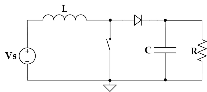
A boost converter is used to transform the low input voltage into the high voltage required by the GM tube.

How the boost converter works

1. Switch closed

When the switch is closed, the current flows through the inductor $L$ rather than through the diode.

The inductor stores energy in its magnetic field.

2. Switch open

When the switch opens, the current through the inductor must continue flowing. The inductor therefore releases its stored magnetic energy.

Its induced voltage adds to the input voltage and transfers energy to the capacitor $C$ and the load.

Relation between $V_s$ and $V_R$

When the switch is closed, the inductor voltage is

$$V_L = V_{in} = L\frac{dI_L}{dt}$$

During the ON state, the increase in inductor current is

$$\Delta I_{L,\text{on}} = \int_0^{T_{\text{on}}} \frac{V_{in}}{L}\,dt = \frac{V_{in}T_{\text{on}}}{L}$$

When the switch is open, the inductor current flows through the diode.

We have

$$V_{in} = V_L + V_R$$

and therefore

$$V_L = V_{in}-V_R = L\frac{dI_{\text{off}}}{dt}$$

During the OFF state:

$$\Delta I_{L,\text{off}} = \int_0^{T_{\text{off}}} \frac{V_{in}-V_R}{L}\,dt = \frac{(V_{in}-V_R)T_{\text{off}}}{L}$$

At steady state, the current through the inductor is the same at the beginning and end of each switching cycle:

$$\Delta I_{L,\text{on}} + \Delta I_{L,\text{off}} =0$$

Thus,

$$\frac{V_{in}T_{\text{on}}}{L} + \frac{(V_{in}-V_R)T_{\text{off}}}{L} =0$$

which gives

$$V_R = \frac{V_{in}}{1-D}$$

with the duty cycle

$$D = \frac{T_{\text{on}}} {T_{\text{on}}+T_{\text{off}}}$$

Therefore, by modifying the duty cycle $D$, the boost converter can increase a low continuous voltage, such as $9\,\text{V}$, to a much higher continuous voltage, such as approximately $400\,\text{V}$.